
Fundamentals of Time Series Database Engineering (TSDB)
#5.1: Fundamentals of designing time series databases with Google's Monarch and Facebook's Gorilla DB

This article is part I of a 2 part series on designing a time series database taking lessons from Monarch and Gorilla DB.
What is a time series database?
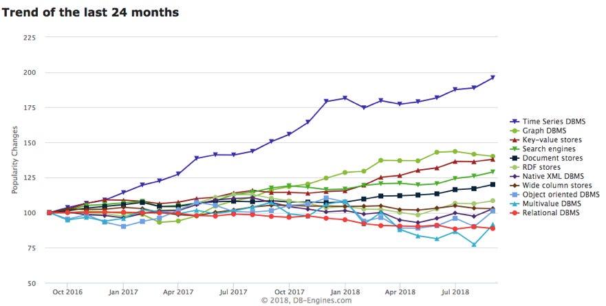
Time Series Database or TSDB is a database optimised for storing and querying time series (or timestamped) data. They are mostly used for querying and analyzing metrics data for different systems. So they need to support complex data analysis quickly and efficiently eg- server metrics, application monitoring, clicks per user, analyzing finance and trading trends etc. Popular examples of TSDB include Prometheus, Influx DB, Gorilla DB and Monarch.
Comparison with general-purpose NoSQL databases
Time series data consist of measurement values of a target, changing over time. We need complex analysis of this data to understand it better. Some examples - For querying a time range, aggregations per x minute like P99 (99th percentile) histograms on the data or Cumulative sum every x minutes. While possible, it can be challenging to tune other NoSQL databases like key-value stores for this purpose.
TSDBs are optimised for batching and compacting writes to support high throughput and have built-in support for aggregations mentioned above. Most metrics also require custom tags to quickly query target data, handled out of the box by TSDBs.
Now that we understand what a TSDB is and its usage, let’s try to design one.
Requirements of a TSDB
Let’s start by looking at the functional and non-functional challenges specific to a TSDB.
Heavy write throughput and spiky read traffic
Ingesting 1000s of systems and application monitoring metrics from a hundred instances of thousands of systems every minute makes up a pretty high write load (Monarch handles TBs of data per second). So TSDB see a very high write load.
The reading load is spiky as and when the databases query for users looking up dashboards or from scheduled searches.
Latest data is the most queried one
As observed at Facebook (and other systems), users are most often concerned only with recent data (up to 2 days). So our TSDB should optimize the data storage so that querying this data is performant.
Huge amount of data
From the 2 above points, we need to persist a huge amount of data (~260TB per month). But since most users are concerned with the latest data (<2 days say) we can downsample our data from per-second granularity to per-minute granularity after a week, and to an hour granularity after a month. This will help in significantly cutting down storage costs.
Aggregations and rollups
Most metric visualization systems require time range-based querying of data and complex analysis of the data like different aggregations on time windows. Our TSDB needs to be able to support this.
Consistency vs availability
We opt for high availability for reads and writes and trade-off consistency in case of network partitioning in the TSDB system. So our system would still accept writes even though it might not be synced to the other nodes in case of a network partition. So our system can drop delayed writes and return partial queries for reads.
Also, our system would be available for reads but it might not have the latest data (may return partial results) and give an indication to the user about it.
Data Collection in Time Series Database
Let’s discuss the different ways client system metric data collection is done in a TSDB.
Push based approach
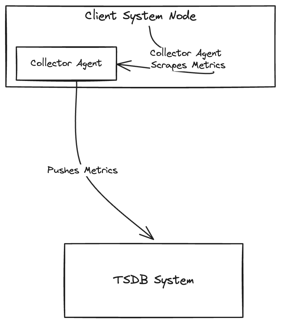
In this approach, a collector agent is installed in the client system nodes. This agent scrapes the metrics data from the system (at the node level) by querying pods, kubectl API etc. and pushes the metrics to the TSDB system. This approach is popularly used by Monarch, Gorilla DB, Graphite etc.
Pros of this approach include:
good for cases where ephemeral jobs need to push metrics and might not be available long enough for a pull-based approach
no service discovery component required
Cons of this approach entail:
anyone can push data to the TSDB, however, this can be avoided by implementing authentication on the TSDB, so only genuine collector agents can push data
the write throughput is not controlled, since a lot of data can be pushed all of a sudden if traffic on the client side increases - this can be handled by aggregating data on the agent side before pushing it to TSDB
Pull based approach
In this approach, the client system exposes a metrics API which is polled by the TSDB at regular intervals.
Pros of this approach include:
the metrics API can be hit using a curl to check the metrics exposed by the system
the rate of pulling data can be maintained at the TSDB level
Cons of this approach entail:
A service discovery component needs to be maintained with TSDB where the clients can register themselves (with host IP and URL) so TSDB knows where to fetch metrics from
Several clients have a firewall layer which needs to be whitelisted for TSDB to fetch data
Aggregation on collection
Data can be aggregated at the client/agent level at a configurable duration before pushing it to the TSDB server. This helps in increasing write throughput to TSDB by reducing individual calls every second and aggregating multiple metrics in one call.
This is especially helpful when tracking per-user metrics from different nodes/ instances for a client system. Ultimately we’re only concerned about the user activity in this case, not the instance that internally handles it.
Gauge metrics vs Cumulative metrics
Gauge metrics are individual metric points tracked for a particular target. It represents a single numerical value that can arbitrarily go up and down. It captures the current value of a particular measurement at a specific point in time.
A cumulative metric represents a value that only ever increases (or resets). It typically counts occurrences of events or accumulates values over time. So cumulative metrics contain information about all the earlier points as well (from a given start time).
We prefer cumulative metrics over gauge metrics wherever possible since even if we lose some data, the next data will contain the cumulative metric including the previously lost point as well.
Examples
While monitoring a web server:
Gauge Metric:
current_active_sessions– shows the number of active sessions at the current moment.Cumulative Metric:
total_requests_served– counts the total number of HTTP requests served by the web server since it started.
Decouple collection and ingestion
If we go ahead with the push-based approach for data collection, we do not have control over the write throughput (even with collection aggregation). To control the ingestion rate to the database/storage layer, we use a queue to decouple collection and ingestion processes. Workers will pull raw metrics from the queue, and push it to the storage layer at a configurable rate.
It is not necessary to use decoupling if the database layer can easily scale to handle the load. Both Monarch and Gorilla DB directly can handle and scale according to the write throughput.
Data Model and Schema
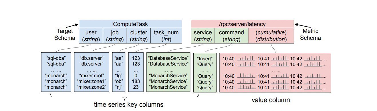
As we discussed above, the data can be any kind of timestamped data with values for a metric. Monarch uses a powerful data model for this data - with a target schema and metric schema for each record. This helps read and write performance by limiting fanout as discussed in the subsequent section.
cpu_usage{host="server-123", region="ap-south1"} 75.5 1689165296789Target Schema
This includes the metadata and labels associated with the metric. Every target has a location field that helps in routing the data for ingestion to the right zone. In the below example, the region defines the location. The target fields are also used for lexicographic sharding during ingestion.
{
  "host": "server-123",
  "region": "us-central1"
}
Metric Schema
This contains the actual metric data - the name, value, and timestamp sent by the clients.
{
  "metric_name": "cpu_usage",
  "timestamp": "2024-07-12T12:34:56.789Z",
  "value": 75.5
}
Data ingestion
In Monarch, data ingested is stored locally (in the same region, but in different clusters for fault tolerance) for better reliability, low transmission costs and low latency.
Data hierarchy
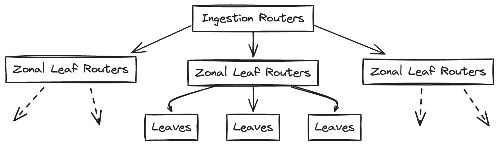
There are 3 layers or levels within the TSDB.
Ingestion Routers: The topmost layer responsible for receiving and routing incoming data.
Zonal Leaf Routers: The middle layer that distributes data to the appropriate storage nodes.
Leaves (Storage Nodes): The bottom layer where the actual time series data is stored.
Data flow during ingestion
The data is sent from the agent installed in the client systems which aggregates the metrics and pushes it to one of the ingestion routers.
The target has information on region, host etc. as seen from the above schema diagram. The ingestion router passes the data to the leaf routers in the relevant zone based on the location field in the target. The location-to-zone mapping is maintained in configuration to ingestion routers.
At the zone level (ie the leaf routers), the data is routed to the relevant leaves based on the range assigned by the range assignor and also maintained within the leaf routers. This range assignment helps to control the fanout - ie only the leaves which store the metric data for the target are involved in ingestion. This ingestion also triggers updates to the root and zone index servers in Monarch.
A point to note here is that Monarch leaves update the range to leaf mapping directly in the leaf routers to maintain the source of truth (ie leaves) and to reduce dependency on the range assignor for writes.
In Monarch and GorillaDB, the data is replicated across different clusters for better fault tolerance. GorillaDB also employs a circuit breaker when a zone goes down. If it is seen as being down for x amount of time, it will direct all queries to the other zones for 48 hours.
Load Balancing across leaves
The range assignor acts as a load balancer, delegating ranges to leaves according to their CPU and memory usage. Range assignment changes dynamically, while collection happens simultaneously:
A new leaf instance (L2) joins the group of leaves in the zone for scaling up. The range assignor identifies a range from an existing leaf (L1) to assign to the new leaf.
The new leaf informs the leaf routers of its assignment, ensuring data for ingestion comes to L1 and L2 for some time. L2 then stores the data in memory, writes recovery files etc.
The L2 leaf waits for 1 second for the L1 leaf to write to its recovery logs, and then begins reading from L1’s recovery logs to keep track of older data.
Once the data transfer from recovery logs is complete for L2, it informs the range assignor to unassign the range from L1. L1 stops collecting data for the range and drops the in-memory data for the range.
Query layer
We can opt for a query service, which would be a thin layer on top of our database layer. This would help in optimising to serve queries to the database. If the database is powerful enough to support data schemas (like in Monarch), we do not need this layer.
Also, data compressed for writes may not be best for serving read queries. This layer can help in improving the performance of read queries. This layer can help prefetch scheduled queries by caching them (like in Gorilla DB, which is a write-through cache on top of the actual TSDB system Facebook has, called ODS).
References
That was all for the fundamentals of designing a time series database!
In part 2 of this series, we will explore the advanced concepts of TSDB Design, including query evaluators, fault tolerance, and data persistence, along with visualization and alerting systems.